
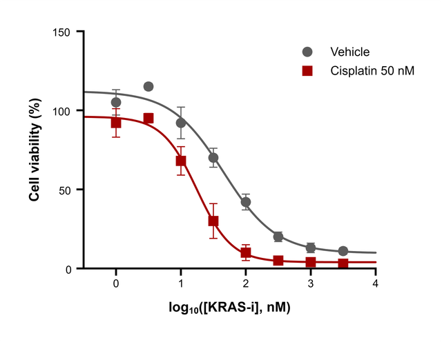
The data you need
An XY table with one concentration per row in X, either the concentration itself or its log10, and the responses of each treatment as a data set. Set Replicates to the number of wells per concentration; every replicate counts in the fit.
What the fit reports
Open the Analysis panel and choose Nonlinear regression (dose–response). For each data set you get:
| Result | Meaning |
|---|---|
| Bottom, Top | The lower and upper plateaus |
| EC50 (the IC50 for an inhibition curve) | The concentration halfway between Bottom and Top, in your units |
| Hill slope | Steepness at the midpoint; negative when the response falls with dose |
| R², Sy.x | How closely the curve follows the points |
Choose log(agonist) vs. response — variable slope when X is log10(concentration), or [Agonist] vs. response — variable slope when X is the concentration itself.
On the graph
Draw fitted curve on graph adds each curve in the color of its data set. Show the concentrations on a log axis with Format Axes → Scale → Log 10, and style the curves under Fitted curves in Format Graph. Each treatment is fitted separately, so their EC50 values can be compared side by side.
Export for a journal
Export the figure as TIFF at up to 1200 dpi, or as PDF, EPS or SVG vector artwork; see How to export a 300 dpi TIFF figure for a journal. Report the IC50 with its unit, for example IC50 = 17.6 nM.
Frequently asked questions
IC50 or EC50? The same parameter under two names: EC50 for a stimulating effect, IC50 for an inhibiting one.
How many concentrations do I need? At least five points that reach both plateaus, ideally spaced evenly on a log scale, such as half-log or 3-fold dilutions.